Quantile regression with LightGBM

TL;DR

LightGBM 은 Microsoft 에서 개발한 gradient boosting tree framework 로 모델 적합이 빠르고 계산량이 적어서 자주 사용된다. LightGBM 에서는 기본적으로 quantile을 추정하는 알고리즘을 내장하고 있다. 그러나, LightGBM에는 무시하지 못할 중대한 결함이 있는데, 이는 마지막에 다루도록 하겠다.

Example

예제에 사용할 데이터는 다음과 같다. 예제는 링크에서 참고했다.

import numpy as np

sample_size = 500
x = np.linspace(-10, 10, sample_size)
y = np.sin(x) + np.random.uniform(-0.4, 0.4, sample_size)
x_test = np.linspace(-10, 10, sample_size)
y_test = np.sin(x_test) + np.random.uniform(-0.4, 0.4, sample_size)

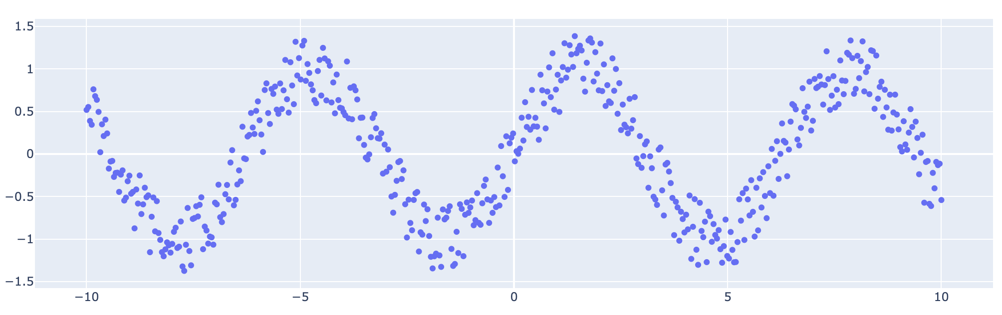
해당 데이터를 간단하게 다음과 같이 시각화 해볼 수 있다.

import plotly.graph_objects as go

fig = go.Figure(go.Scatter(x=x, y=y, mode="markers"))
fig.show()

LightGBM 에서는 기본적으로 Quantile을 추정하는 옵션을 제공한다. 이는 다음의 두 가지 옵션을 통해 가능한데

• params에 “objective”를 “quantile”로 설정,
• “alpha”로 원하는 quantile 을 입력,

하는 방식이다. 예를 들어, 아래는 Median("alpha" : 0.5)을 추정하는 모델의 구성이다.

import lightgbm as lgb

params = {
    "objective": "quantile",
    "alpha": 0.5,
    "max_depth": 4,
    "num_leaves": 15,
    "learning_rate": 0.1,
    "n_estimators": 100,
    "boosting_type": "gbdt",
}

x_reshaped = x.reshape(-1, 1)
train_dataset = lgb.Dataset(data=x_reshaped, label=y_train)
model = lgb.train(
    train_set=train_dataset,
    verbose_eval=False,
    params=params,
)

생성된 모델에 대해서 예측도 굉장히 단순하다. 다음과 같이 model의 predict method를 사용하면 된다.

x_test_reshaped = x_test.reshape(-1, 1)
preds = model.predict(data = x_test_reshaped)

마지막으로, y_test와 preds를 한 그래프에 시각화하여 결과를 확인해보자.

import plotly.graph_objects as go

fig = go.Figure(
    go.Scatter(
        x=x_test,
        y=y_test,
        mode="markers",
        name="test",
    )
)
fig.add_trace(
    go.Scatter(
        x=x_test,
        y=preds,
        name="predict"
    )
)
fig.show()

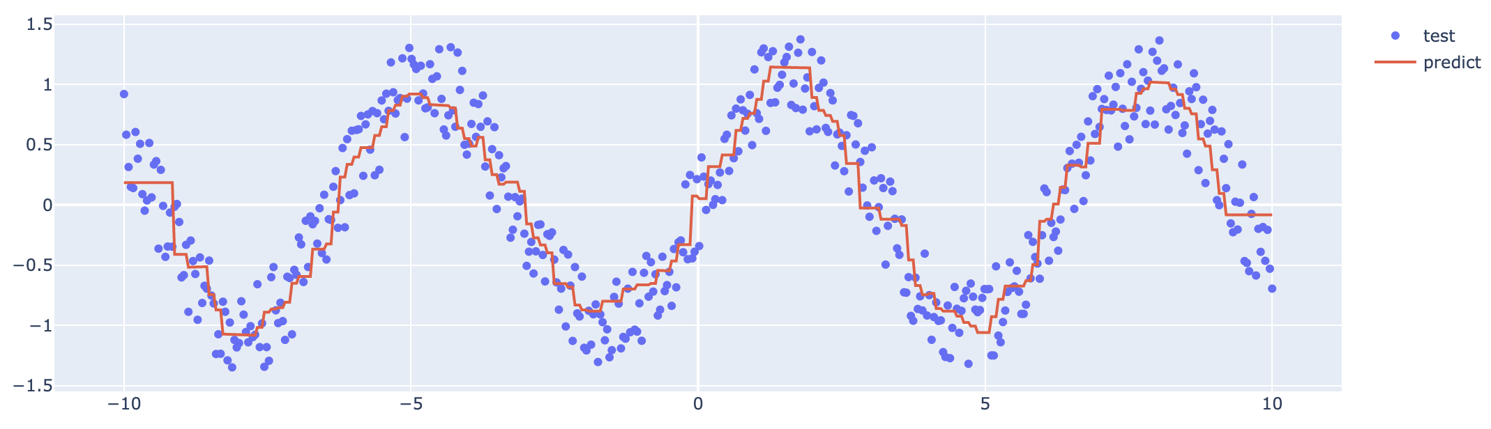
양쪽 끝에 이상한 형태가 보이지만 애써 무시한다. 위처럼 LightGBM은 단순하고 빠르게 quantile을 추정할 수 있는 framework이다. 그러나, 문제는 여러 개의 quantile을 동시에 추정할 때 발생한다.

Problem

여러개의 quantile을 추정하는 문제, 혹은 Prediction Intervals을 추정한다고 표현하기도 한다, 를 해결하기 위한 대안으로 몇 개의 문서가 있다 (Scikit learn 예제 글, IBM 글, Towardscience 글). 세 문서의 골자는 다음과 같다. 각 quantile 마다 모델을 다르게 학습하라는 것이다.

alphas = [0.1, 0.2, 0.3, 0.4, 0.5, 0.6, 0.7, 0.8, 0.9]
train_dataset = lgb.Dataset(data=x_reshaped, label=y_train)
model_list = []
for alpha in alphas:
    params = {
        "objective": "quantile",
        "alpha": alpha,
        "max_depth": 4,
        "num_leaves": 15,
        "learning_rate": 0.1,
        "n_estimators": 100,
        "boosting_type": "gbdt",
    }
    model_list.append(
        lgb.train(
            train_set=train_dataset,
            verbose_eval=False,
            params=params,
        )
    )

이는 자세히 생각해보면 굉장히 잘못된 접근이라는 것을 알 수 있다. Quantile 의 정의에 의해 낮은 quantile 예측값은 높은 quantile 예측값보다 작아야만 한다. 그러나, 해당 접근은 이 부분이 결여되어 있다. 직접 추정값으로 확인해보자.

preds_list = [model.predict(x_test_reshaped) for model in model_list]
preds_df = pd.DataFrame(preds_list).T
preds_df.loc[(preds_df.diff(axis = 1) < 0).sum(axis = 1) > 0]

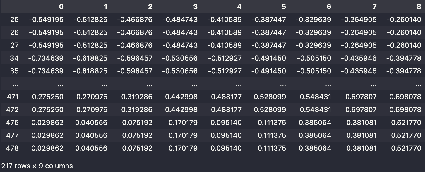
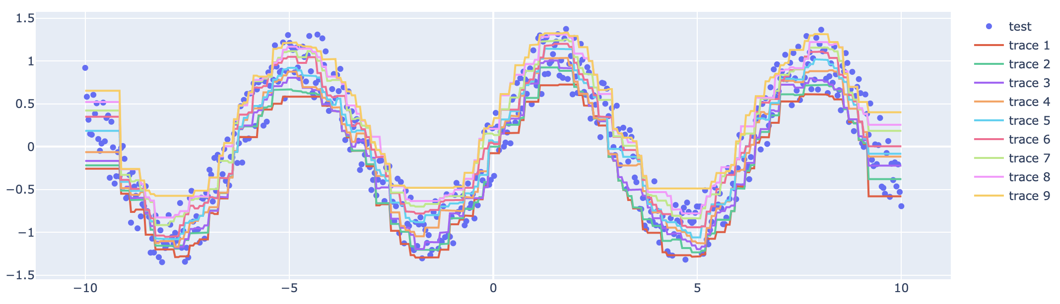
위처럼 500개의 데이터 중에 40%를 넘는 데이터가 순서관계가 어긋나 있음을 확인할 수 있다. 알아보긴 힘들지만, 아래처럼 각 test 데이터에 대해 quantile을 같이 시각화할 수 있다.

import plotly.graph_objects as go

fig = go.Figure(
    go.Scatter(
        x=x_test,
        y=y_test,
        mode="markers",
        name="test",
    )
)
for preds in preds_list:
    fig.add_trace(
        go.Scatter(
            x=x_test,
            y=preds,
        )
    )

fig.show()

Conclusion

다음 글에서는 위에서 발생한 역전 문제 (Crossing problem)을 어떻게 방지할 수 있는지에 대해서 소개하도록 하겠다.